Introduction to Dynamic Programming

Dynamic programming is one of the core algorithmic techniques in all of computer science. It is a very general technique that can be applied to many problems. I chose to write a blog post on this topic because it is the perfect sweet spot of a technique that is surprisingly useful, and one where visual intuition can be core to understanding.

The principle is simple:

Express your problem in terms of overlapping subproblems.
Solve the subproblems, and save the solution.
If the subproblem is ever seen again, you return the saved solution rather than computing it again.

If you have seen Pascal’s triangle before, you have seen dynamic programming.

Pascal’s triangle is generated by a simple recurrence relation: each digit is the sum of the two digits directly above it. Another representation of Pascal’s triangle is in a table, as follows:

1	1	1	1
1	2	3	4
1	3	6	10
1	4	10	?

What if I asked you what the value is in the bottom right corner of the table? It’s obviously 20, which is the sum of digits above and to the left of the digit. But importantly, this was only easy because you had access to a table, and most of it was filled in already.

This is exactly the crux of dynamic programming: table-filling.

Here’s a challenge: try to find that same value, with the constraint that you can’t use a table of any sort (this includes writing down the triangle). It’s much harder, and extremely tedious to do (note that $P_{i,j}$ represents the value of the $i$ -th row and $j$ -th column):

$\begin{aligned} P_{4,4} &= P_{3,4} + P_{4,3} \\ &= (P_{2,4} + P_{3,3}) + (P_{3,3} + P_{4,2}) \\ &= ((P_{1,4} + P_{2,3}) + (P_{2,3} + P_{3,2})) + ((P_{2,3} + P_{3,2}) + (P_{3,2} + P_{4,3})) \\ &= \cdots \\ &= 1 + 1 + 1 + ... + 1 \\ \end{aligned}$

Notice that in this computation, many values appeared more than once (for example, $P_{3,3}$ and $P_{2,3}$ ). This is exactly what is meant by overlapping subproblems. The key idea is that once you solve the subproblem once, you don’t need to solve it again. Just save the value, and return that value the next time you need it. With this framework, it is possible to achieve huge speedups.

The Fibonacci sequence

The Fibonacci sequence is a commonly used example when first teaching about dynamic programming. It has the following recursive definition:

$\begin{aligned} \text{Fibonacci}(n) &= \text{Fibonacci}(n-1) + \text{Fibonacci}(n-2) \\ \text{Fibonacci}(1) &= 1 \\ \text{Fibonacci}(2) &= 1 \\ \end{aligned}$

The task is, calculate the value of $\text{Fibonacci}(1000)$ .

Brute Force Solution

The natural solution, then, if you’re doing it in Python, would be to write it like so:

def fibonacci(n):
    if n <= 2:
        return 1
    else:
        return fibonacci(n-1) + fibonacci(n-2)

While this produces the correct answer, it is much too slow. In fact, the amount of time needed to produce the correct answer is exponential in the input size.

(I generated the plot with this code).

The reason for this is that each call to fibonacci makes two more calls to fibonacci, and hence, twice the amount of addition must be done. For large values of n, this creates an exponential amount of work.

DP Solution

Instead, let’s treat the problem like filling up a table. This table would only have one dimension, which represents the value of $n$ , and its value would represent $\text{Fibonacci}(n)$ . We can fill the table like so:

Notably, the amount of addition is linear with $n$ , rather than being exponential in $n$ . This is a massive improvement! The corresponding Python implementation would look something like this:

def fibonacci(n):
    table = [1, 1]

    while len(table) < n:
        table.append(table[-1] + table[-2])

    return table[-1]

And as can be seen by the following plot, this leads to a massive speedup. Values of $n$ much larger than 100,000 can be calculated in under a second. And more importantly, the shape of this curve is roughly linear, so this method scales very well to high $n$ .

Tri-tiling

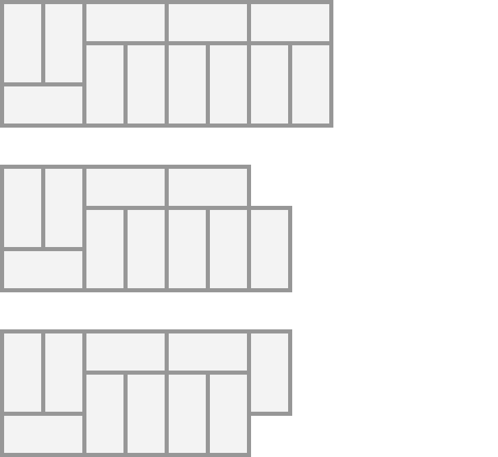
Let’s try a slightly more difficult problem. Given a $(3 \times n)$ board, find the number of ways to fill it with dominoes of length 2. Here is one possible solution:

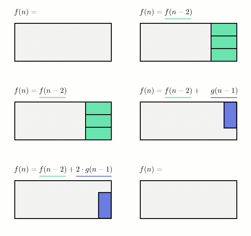
First, we start by defining a subproblem $D_n$ which represents the number of tilings of a board of length $n$ . This time, though, the recurrence relation is significantly more tricky, because you can end up with intermediate boards of two different forms:

Observations

The only intermediate forms which are valid either are completely filled at the end, or have one empty hole at a corner.
It is not possible to have a fully-tiled board of odd length (try for yourself).
Also, other intermediate forms (two empty squares on the corners, one empty square in the center) are not valid intermediate solutions either.

Recurrence

What if instead of using just one recurrence relation, we used multiple recurrence relations, one for each intermediate solution type?

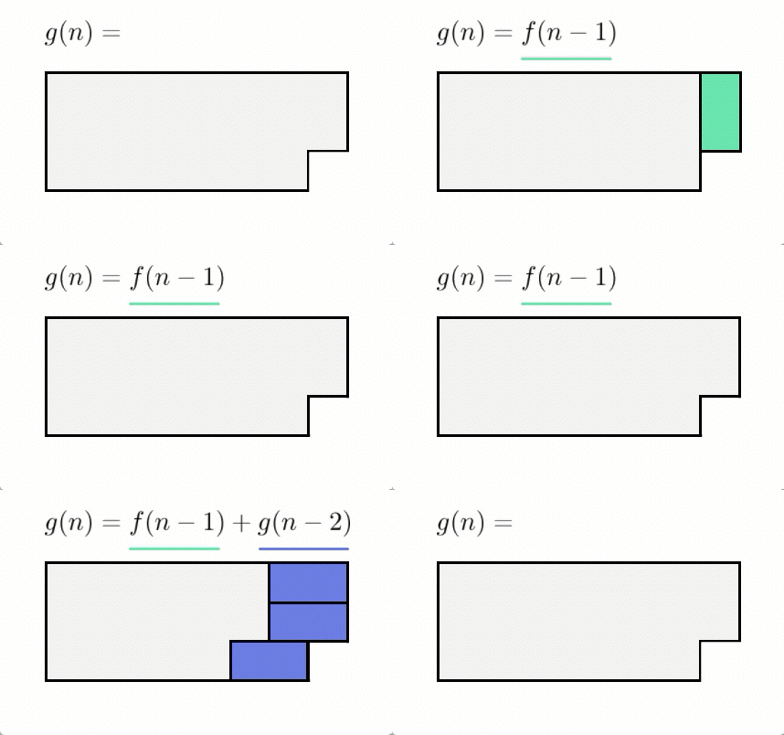
Let’s call $f(n)$ the number of ways to tile a $(3 \times n)$ board such that it has a flat end, and $g(n)$ the number of ways to tile a $(3 \times n)$ board such that it has one corner missing.

Also note that our base cases for $f$ are $f(0) = 1$ , since there is only one way to tile an empty board, and $f(1) = 0$ , since it is impossible to tile a board of length 1. We can also express $g(x)$ recursively:

With base cases $g(0) = 0$ , since there are no ways to tile zero spots with a missing square, and $g(1) = 1$ , since you can make one tiling with a missing square in a $(1 \times 3)$ board.

To reiterate, we get the following recurrence relations:

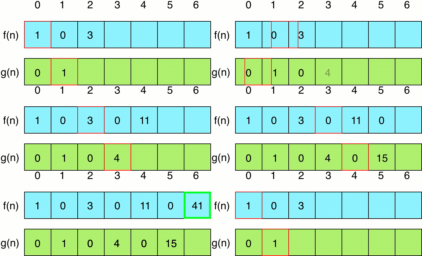
$\begin{aligned} f(n) &= f(n-2) + 2*g(n-1) \\ f(0) &= 1 \\ f(1) &= 0 \\ \\ g(n) &= f(n-1) + g(n-2) \\ g(0) &= 0 \\ g(1) &= 1 \\ \end{aligned}$

This means that this is what our table-filling algorithm would look like this:

Notice that we alternate between finding values of $f(x)$ and $g(x)$ . This illustrates the fact that DP algorithms can fill tables in complex ways. The one invariant, though, is that tables must be filled from left to right or top to bottom. This corresponds to the fact that larger solutions must consist of smaller solutions. Our corresponding Python function might look like this:

def tri_tiling(n):
    f = [1, 0]; g = [0, 1]
    
    while len(f) <= n:
        next_f = f[-2] + 2*g[-1]
        next_g = f[-1] + g[-2]
        f.append(next_f)
        g.append(next_g)
    
    return f[n]

Note that we store our values in intermediate variables, because otherwise we would be modifying the length of the array and hence in the next_g line we would get the wrong value from f[-1].

As you can see, dynamic programming can be an incredibly powerful paradigm. Even simple linear table-filling algorithms like the one presented for Fibonacci can make an exponential algorithm run in linear time. As was shown in the second example, there can be a large amount of variety in how values are constructed from previous values. In my next post, I will cover dynamic programming algorithms that operate on two-dimensional tables and even trees.