Dynamic Programming in Policy Iteration

Richard Bellman was a man of many talents. In addition to introducing dynamic programming, one of the most general and powerful algorithmic techniques used still today, he also pioneered the following:

The Bellman-Ford algorithm, for computing single-source shortest paths
The term “the curse of dimensionality”, to describe exponential increases in search space as the number of parameters increases
Many contributions to optimal control theory, artificial intelligence, and reinforcement learning.

In this post, I’m going to focus on the latter point - Bellman’s work in applying his dynamic programming technique to reinforcement learning and optimal control. He introduced one of the most fundamental algorithms in all of artificial intelligence — that of policy iteration.

Value iteration is a method of finding an optimal policy given an environment and its dynamics model. I’ll describe in detail what this means later, but in essence what this means is that due to Richard Bellman and dynamic programming it is possible to compute an optimal course of action for a general goal specified by a reward signal. This launched the field of reinforcement learning, which has recently seen some notably huge successes with AlphaGo Zero and systems which can learn to play complicated games directly from pixels.

This post is not a tribute to Richard Bellman, but he was a truly incredible computer scientist and someone whose life I find truly inspiring.

Markov Decision Processes

A Markov Decision Process (MDP) is a general formalization of decision making in an environment.

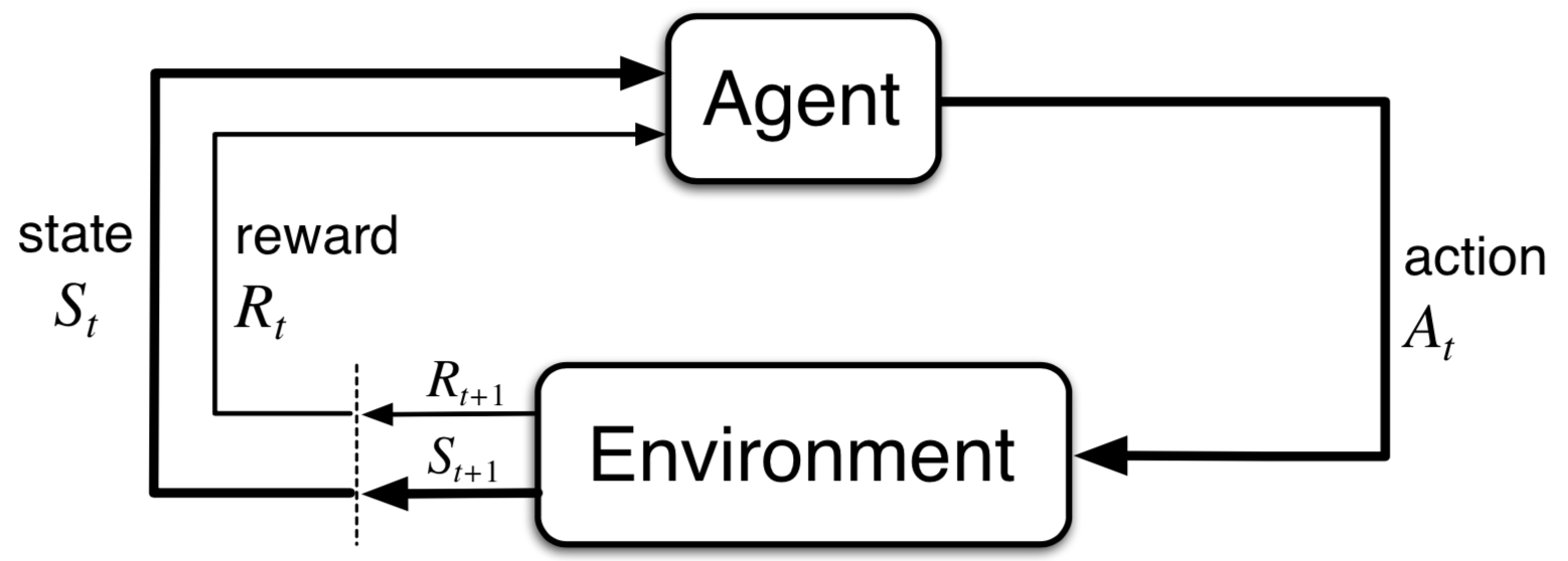
In reinforcement learning, there is an agent acting in an environment. At every iteration, an agent is acting in the environment. This agent sees the current state of the MDP, and based on this state it must choose some action. Once this action is taken, it sees the next state and it may receive some positive or negative reward. The goal of the agent is to act so as to maximize the total reward it receives. Here’s a specific example of what such an MDP might look like.

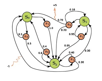
In this example, each of the green circles represent a state, so the set of states $\mathcal{S} = \{S_0, S_1, S_2\}$ . Each of the red circles represents an action available in that state, so the set of actions $\mathcal{A} = \{a_0, a_1\}$ . Moreover, note that a given action in some state may end up in more than one state, denoted by a probability associated with each arrow. These probabilities are given by some transition model $\mathcal{T}$ :

$\mathcal{T} = P_a(s, s') = \Pr(s_{t+1} = s' | s_t = s, a_t = a)$

For example, $P_{a_0}(S_1, S_0) = 0.70$ and $P_{a_0}(S_1, S_2) = 0.20$ . Finally, the yellow emitted lines represent rewards given on a state transition. Note that these rewards are associated with a state-action pair, and not just a state. These are given by the reward function $\mathcal{R} = R_a(s, s')$ which is dependent on a state-action pair.

It is up to the agent to act in such a way to see highly positive rewards often, and to minimize the number of highly negative rewards it encounters.

Let us come up with a formalization of this goal of the agent. We define a (deterministic) policy $\pi$ to be a mapping from state to action, that is:

$\pi(a | s) = \begin{cases} 1 \text{ if action $a$ is taken in state $s$} \\ 0 \text{ otherwise} \end{cases}$

A natural goal would be to find a policy $\pi$ that maximizes the expected sum of total reward over all timesteps in the episode, also known as the return $G_t$ :

$G_t= R_t + R_{t+1} + R_{t+2} + \cdots = \sum_{k = 0}^T R_{t+k}$

Where $T$ denotes timestep of the end of the episode. Unfortunately, in some cases we might want $T$ to be $\infty$ , that is, the episode never ends. In this case, the sum would be an infinite sum and would diverge. To remedy this problem, we introduce a discount factor $\gamma$ such that each reward gets weighted by a multiplicative term which is between 0 and 1:

$G_t = R_t + \gamma R_{t+1} + \gamma^2 R_{t+2} + \cdots = \sum_{k=0}^\infty \gamma^k R_{t+k}$

Since our return may be different every time, because taking the same action in a given state may lead to different results according to the transition model, we want to maximize the expected cumulative discounted reward. This is known as the optimal policy $\pi^*$ :

$\pi^* = \max_\pi \mathop{\mathbb{E}}_\pi \left[ \sum_{k=0}^T \gamma^k R_{t+k} \right]$

This is the reinforcement learning problem. Given an MDP as a 5-tuple $(\mathcal{S}, \mathcal{A}, \mathcal{T}, \mathcal{R}, \gamma)$ , find the optimal policy $\pi^*$ that maximizes expected cumulative discounted reward.

Value Iteration

The policy iteration algorithm computes an optimal policy $\pi^*$ for an MDP, in an iterative fashion. It has been shown to converge to the optimal solution quadratically — that is, the error minimizes with $\frac{1}{n^2}$ where $n$ is the number of iterations. This algorithm is closely related to Bellman’s work on dynamic programming.

Value functions

Before we describe the policy iteration algorithm, we must establish the concept of a value function. A value function gives a notion of, on average, how valuable a given state is. A value function answers the question, “what is the reward I should expect to get from being in a given state?”. Formally, a value function is defined to be:

$v_\pi(s) = \mathop{\mathbb{E}}_\pi \left[ G_t | S_t = s \right]$

In other words, the value function defines the average return given that you start in a given state and continue forward with the policy $\pi$ until the end of the episode.

The Bellman equation

Importantly, Bellman discovered that there is a recursive relationship in the value function. This is known as the Bellman equation, which is closely related to the notion of dynamic programming:

$v_\pi(s) = \mathop{\mathbb{E}}_\pi \left[ R_t + \gamma G_{t+1} | S_t = s \right]$

Ideally, we want to be able to write $v_\pi(s)$ recursively, in terms of some other $v_\pi(s')$ values for some other states $s'$ . This would allow us to recursively find the value function for a given policy $\pi$ . It turns out that the recursive formulation is exactly this:

$v_\pi(s) = \sum_{a \in \mathcal{A}} \pi(s | a) \underbrace{\left[ \sum_{s' \in \mathcal{S}} \sum_{r} \overbrace{p(s', r | s, a)}^\text{prob. of state-action} \underbrace{\left[r + \gamma v_\pi(s') \right]}_\text{value of state-action} \right]}_\text{expected value of action $a$ in state $s$}$

Visually, it may look like there’s a lot going on in this recursive formulation, but all it’s doing is performing an expected value over actions of the expected return from that action. Each expected value of an action is itself an expected value over possible next states and rewards. Using this equation, we can easily derive an iterative procedure to calculate $v_\pi(s)$ .

The policy iteration algorithm

The main idea is that this can be done in an iterative procedure. At every iteration, a sweep is performed through all states, where we compute:

$v_\pi(s) = \sum_{a} \pi(s | a) \sum_{s'} \sum_{r} p(s', r | s, a) \left[r + \gamma v_\pi(s') \right]$

Note that if we are given the MDP $(\mathcal{S}, \mathcal{A}, \mathcal{T}, \mathcal{R}, \gamma)$ , as well as some policy $\pi$ , this is something we have all the pieces to compute. As we perform this iteratively, the changes in value function will become smaller and smaller and will eventually converge (quadratically) at the true $v_\pi$ . Of course, we can’t perform an infinite number of iterations, so typically we just say that if the total change of the value function is below some small threshold, stop the procedure.

A worked-through example—grid world

Let’s say that we have some grid, and our agent can move in any direction. We define the grid world with a reward of +1 at the top right corner, and -1 at the bottom right corner. Once an agent reaches one of these corners, the episode ends. This looks like this:

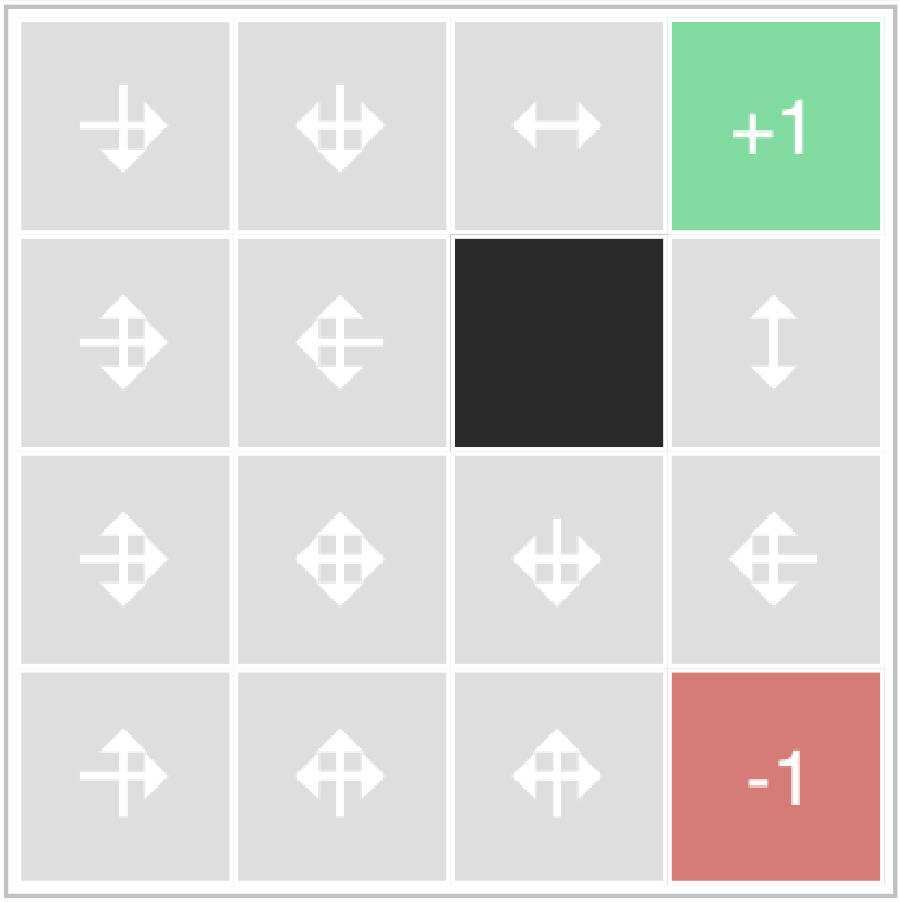
Notice also how there is a wall in the middle of the map, which prevents movement in that direction. Notably, here we are going to say that the discount factor $\gamma = 1$ , and there is no noise - that is, each action deterministically takes the agent to the next state pointed to by the arrow.

For now, let’s define our policy $\pi_0$ to be the policy that moves in any valid direction with equal probability. This is known as the equiprobable policy.

In value iteration, at every iteration then, each state’s value will become the average of the states surrounding it. This table-filling behavior will converge to the correct value function, $v_{\pi_0}$ , as can be seen in the following animation:

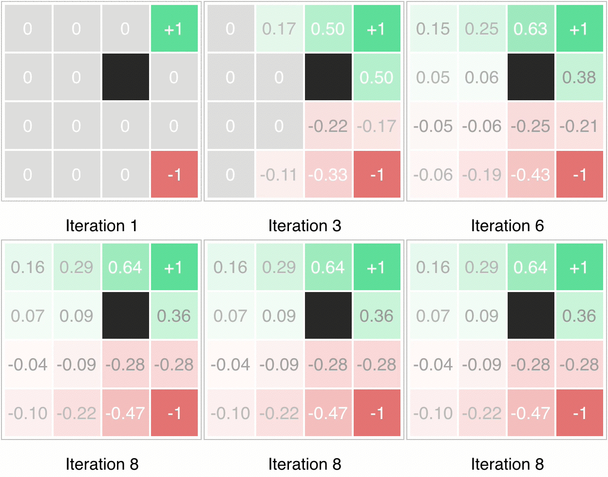
Notice how this is a special case of dynamic programming, which fills a table which is in the shape of the environment. We can then perform policy improvement by greedily improving the policy with respect to the new value function.

$\pi_{t+1}(a | s) = \arg \max_a \sum_{s'} \sum_r p(s', r | s, a) \left[r + \gamma V(s') \right]$

Since our environment is deterministic, $p(s', r | s, a)$ is $1$ where the arrow points, and $0$ everywhere else. Also, since $\gamma = 1$ and $r = 0$ everywhere but the terminal states, the policy improvement update greedily chooses the direction which maximizes the value of the future state. This can be seen graphically here:

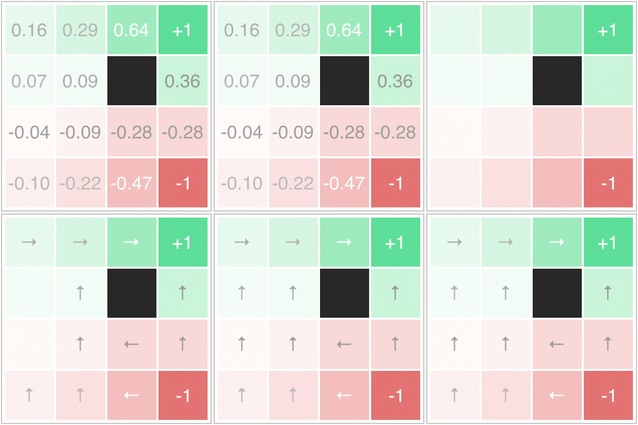
Now this policy could be evaluated, and we could alternate between policy evaluation (finding a value function for $\pi_t$ ) and policy improvement (greedification of the policy with respect to the value function):

$\pi_0 \xrightarrow{E} v_{\pi_0} \xrightarrow{I} \pi_1 \xrightarrow{E} v_{\pi_1} \xrightarrow{I} \cdots \xrightarrow{I} \pi_* \xrightarrow{E} v_{\pi_*}$

And, as can be seen, we would eventually reach the optimal policy $\pi_*$ and value function $v_{\pi_*}$ for the environment. Note that this policy that was found for the environment in one iteration of the algorithm did not find the shortest path to the positive reward. If we wanted to do this, we would need to modify our MDP to encourage this. We could have done this in two ways:

Add in a discount factor $\gamma < 1$ such that states closer to the reward state will have a higher discounted reward than further states
Add in a constant, small negative reward of $-0.1$ for every timestep where the reward is not reached.

Then, the algorithm would find a shortest path to the positive reward terminal state.

Policy iteration is one of the foundational algorithms in all of reinforcement learning and learning optimal control. We introduced the concepts of a Markov Decision Process (MDP), such as expected discounted reward, and a value function. We then informally derived the algorithm for policy iteration, and showed visually how it finds the optimal policy and value function.